Getting ready for machine learning - cleaning up free NHL game and odds datasets
Before beginning any feature engineering or ML, it’s necessary to clean up the data first. In this article we work through a real-life example
Fantasy Football draft season is beginning once again. In past seasons, consistent with the majority of peers in my leagues, my personal draft rankings have been based on expert rankings (and beer sheets), tips from /r/fantasyfootball, and my own intuitions. This year, I’d like to explore a more analytics-driven focus.
My initial plan is to focus on freely-available standard stats (eg Touchdowns, Fumbles, etc) before shelling out for fancy advanced stats websites. I’d like to understand how much past results can predict future results with just simple stats first, to understand if it’s even worth exploring historical stats. My intuition tells me that so much can change year-over-year: injuries, strength of schedule, teammates (eg offensive line for QB/RB, QB for a WR, etc), snap shares, etc. I will not be accounting for any of that in my first iteration.
I’ll be using historical data from footballdb.com and machine learning to predict the expected fantasy points in 2020, based on their stats from 2016-2019. I am targeting 2020 rather than 2021 because we can compare the predicted vs actuals, and using QBs because intuitively I feel that they have a smaller variation year-over-year than other positions such as RBs and WRs. I will not go through all the boilerplate but the full jupyter notebook is available here.
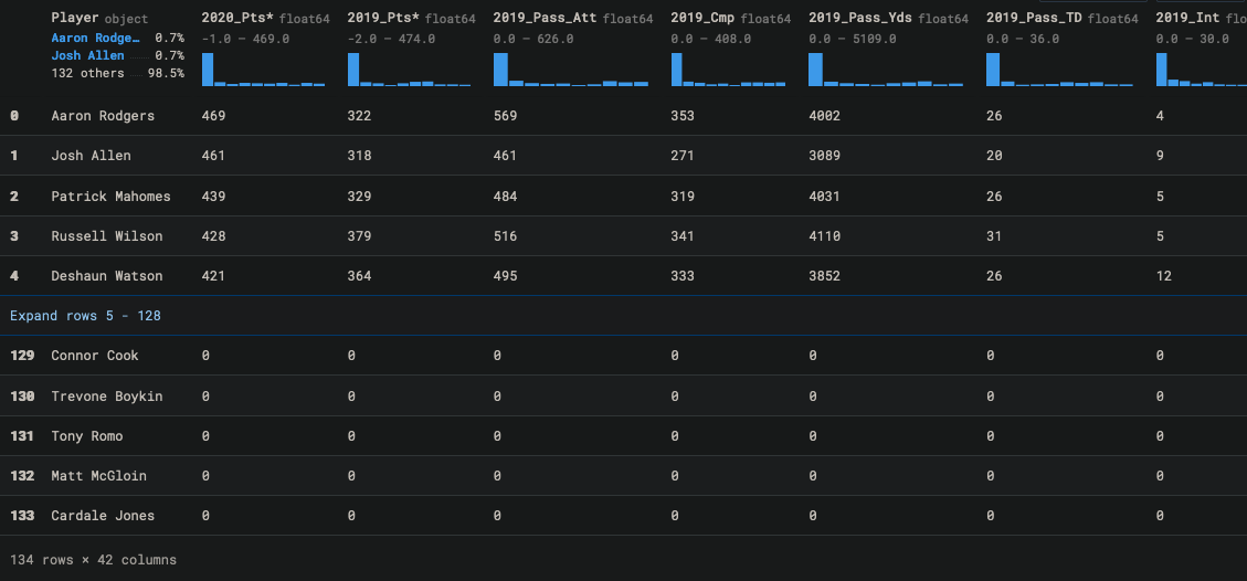
My first plan of action is to pull in data from 2016-2020, and group it by player name. There is some data cleanup required here, specifically that there are duplicate column names depending on category (eg rushing TDs vs passing TDs). I am also doing some feature engineering by dropping columns that won’t have much value (eg fumbles, 2PT conversions). I then need to drop all 2020 columns except for the 2020 fantasy points column. The 2020 fantasy points column will be my target column, and I can’t train the model on 2020 actual data such as touchdowns as that is technically ‘future data’.
# Clean/Merge all the data

year = 2020

# Clean up duplicate columns
# Drop columns that are likely not important based on football knowledge
for i in range(len(qb_data_years)):
    qb_data_years[i] = qb_data_years[i] \
        .rename(columns={"Att": "Pass_Att", "Yds": "Pass_Yds", "TD": "Pass_TD","Att.1": "Rush_Att", "Yds.1": "Rush_Yds", "TD.1": "Rush_TD"}) \
        .drop(columns=["Bye", "2Pt", "2Pt.1", "Rec", "Yds.2", "TD.2", "2Pt.2", "TD.3"])

    column_names = qb_data_years[i].columns.delete(0)
    for column in column_names:
        qb_data_years[i][column] = qb_data_years[i][column].astype(float)
        qb_data_years[i] = qb_data_years[i].rename(columns={column: str(year) + "_" + column})

    year -= 1

merged = reduce(lambda left,right: pd.merge(left,right, on=['Player'], how="outer"), qb_data_years).fillna(0)
# Drop all 2020 columns except points, as those will throw off the testing
merged = merged.drop(columns=["2020_Pass_Att", "2020_Cmp", "2020_Pass_Yds", "2020_Pass_TD", "2020_Int", "2020_Rush_Att", "2020_Rush_Yds", "2020_Rush_TD", "2020_FL"])

That will now give me a dataframe of each player’s stats from 2016-2019, as well as the 2020 points as my target.
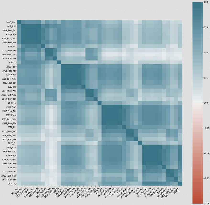
At this point, I stepped back for a bit to look into some correlation data. I’d like to know how well some of the older data correlates to the 2020 points data. If there is a weak correlation, it may be worth dropping the columns to simplify the model.
corr = merged.corr()
plt.figure(figsize=(20,20))
ax = sns.heatmap(
    corr,
    vmin=-1, vmax=1, center=0,
    cmap=sns.diverging_palette(20, 220, n=200),
    square=True
)
ax.set_xticklabels(
    ax.get_xticklabels(),
    rotation=45,
    horizontalalignment='right'
)

It is evident that the 2016 and 2017 data barely correlates to the 2020 points value. This implies that so much can happen in just a couple seasons that it is generally not worth looking at this data.
Moving forward, I created a new dataframe with only 2018 and 2019 data. I also renamed some of the columns to remove the ‘*’ from the 2020 points column (this was from footballdb.com) and put the _year at the end of the column name in order to simplify interacting with pandas later.
year = 2020

# Clean up duplicate columns
# Drop columns that are likely not important based on football knowledge
for i in range(len(qb_data_years_2)):
    qb_data_years_2[i] = qb_data_years_2[i] \
        .rename(columns={"Pts*" : "Pts", "Att": "Pass_Att", "Yds": "Pass_Yds", "TD": "Pass_TD","Att.1": "Rush_Att", "Yds.1": "Rush_Yds", "TD.1": "Rush_TD"}) \
        .drop(columns=["Bye", "2Pt", "2Pt.1", "Rec", "Yds.2", "TD.2", "2Pt.2", "TD.3"])

    column_names = qb_data_years_2[i].columns.delete(0)
    for column in column_names:
        qb_data_years_2[i][column] = qb_data_years_2[i][column].astype(float)
        qb_data_years_2[i] = qb_data_years_2[i].rename(columns={column: column + "_" + str(year)})

    year -= 1

merged_2 = reduce(lambda left,right: pd.merge(left,right, on=['Player'], how="outer"), qb_data_years_2).fillna(0)
# Drop all 2020 columns except points, as those will throw off the testing
merged_2 = merged_2.drop(columns=["Pass_Att_2020", "Cmp_2020", "Pass_Yds_2020", "Pass_TD_2020", "Int_2020", "Rush_Att_2020", "Rush_Yds_2020", "Rush_TD_2020", "FL_2020"])
Then, using a GradientBoostingRegressor, I split up my train and test data and used gp_minimize from skopt to optimize my hyperparameters:
# Get the training data
train_data = merged_2.drop(["Player", "Pts_2020"],axis=1)
target_label = merged_2["Pts_2020"]

# Time to optimize the hyperparameters

n_features = train_data.shape[1]
x_train, x_test, y_train, y_test = train_test_split(train_data, target_label, test_size = 0.30)

clf = ensemble.GradientBoostingRegressor(n_estimators=50, random_state=0)

space  = [Integer(1, 15, name='max_depth'),
          Real(10**-5, 10**0, "log-uniform", name='learning_rate'),
          Integer(1, n_features, name='max_features'),
          Integer(2, 100, name='min_samples_split'),
          Integer(1, 100, name='min_samples_leaf')]

@use_named_args(space)
def objective(**params):
    clf.set_params(**params)

    return -np.mean(cross_val_score(clf, x_train, y_train, cv=5, n_jobs=-1,
                                    scoring="neg_mean_absolute_error"))

clf_gp = gp_minimize(objective, space, n_calls=50, random_state=0)

print(clf_gp.fun)
print("""Best parameters:
- max_depth=%d
- learning_rate=%.6f
- max_features=%d
- min_samples_split=%d
- min_samples_leaf=%d""" % (clf_gp.x[0], clf_gp.x[1],
                            clf_gp.x[2], clf_gp.x[3],
                            clf_gp.x[4]))

clf.fit(x_train, y_train)
clf.score(x_test, y_test)
Depending on the randomization of the test data, this produced an R^2 score of 0.28-0.42, which is very poor. As expected, looking at just a couple years (or more) of basic stats isn’t a great predictor of a QBs future performance. No wonder expert rankings can be so wildly inaccurate! Intuitively I believe that in-season factors are a much larger predictor of performance. In the next post, I’ll explore using factors such as strength of schedule to see if they can improve the model.
Before beginning any feature engineering or ML, it’s necessary to clean up the data first. In this article we work through a real-life example
Discovering several profitable trends that consistently produce positive returns yearly
Leveraging historical performance and spread data to predict what team will cover the spread
昨日はカナダの選挙でした。人気ではありませんでした。
Comparing at the over/under line from 2010 with weather, team ratings, weeks, etc
A review of Matt Rudnitsky’s ‘Smart Sports Betting: How to Shift from Diehard Fan to Winning Gambler’
64% percent of stocks underperform the market and only 6.1% will outperform by 500%+. What makes these outperformers unique?
Using standard QB stats from 2016-2019, teammate ratings, and strength of schedule to predict 2020 fantasy points.
Using standard QB stats from 2016-2019 to compare predicted 2020 fantasy points vs actual performance.
雪が降っていて、桜はアイスクリームみたい
来週、ユダヤの祝日のハヌカーです。
毎年、北米で人気のゲームFantasy Footballをプレイしています。
Available on iOS, Android, BlackBerry, and Web, Red Sea Rescue is a passover themed game using tilt controls to avoid obstacles.
EZ4X is a graphical, automated forex paper trader that allows users to choose techincal indicators and risk tolerance to automatically execute trades on a cu...