Getting ready for machine learning - cleaning up free NHL game and odds datasets
Before beginning any feature engineering or ML, it’s necessary to clean up the data first. In this article we work through a real-life example
In the last post I found that just looking at the last 2-3 years of historical basic stats was not sufficient to predict future fantasy results, and any data older than that was irrelevant. I then theorized that, based on my football intuition, looking at in-season stats like strength of schedule and strength of teammates are more relevant.
Again, the full boilerplate is available in the jupyter notebook here.
year = 2020

# Clean up duplicate columns
# Drop columns that are likely not important based on football knowledge
for i in range(len(qb_data_years)):
    qb_data_years[i] = qb_data_years[i] \
        .rename(columns={"Pts*" : "Pts", "Att": "Pass_Att", "Yds": "Pass_Yds", "TD": "Pass_TD","Att.1": "Rush_Att", "Yds.1": "Rush_Yds", "TD.1": "Rush_TD"}) \
        .drop(columns=["Bye", "2Pt", "2Pt.1", "Rec", "Yds.2", "TD.2", "2Pt.2", "TD.3"])

    column_names = qb_data_years[i].columns.delete(0)
    for column in column_names:
        qb_data_years[i][column] = qb_data_years[i][column].astype(float)
        qb_data_years[i] = qb_data_years[i].rename(columns={column: column + "_" + str(year)})

    year -= 1

merged = reduce(lambda left,right: pd.merge(left,right, on=['Player'], how="outer"), qb_data_years).fillna(0)
# Drop all 2020 columns except points, as those will throw off the testing
merged = merged.drop(columns=["Pass_Att_2020", "Cmp_2020", "Pass_Yds_2020", "Pass_TD_2020", "Int_2020", "Rush_Att_2020", "Rush_Yds_2020", "Rush_TD_2020", "FL_2020"])
Once again I pulled in 2020-2018 data and merge them into a single dataframe. I then pulled in strength of schedule data and merged it in with the main dataframe. This time, I’m keeping the team_2020 column because I’ll need it later.
merged = pd.merge(merged, teams_2019, how="outer").dropna()
merged = merged.rename(columns={"Team" : "Team_2019"})
merged = pd.merge(merged, teams_2020, how="outer").dropna()
merged = merged.rename(columns={"Team" : "Team_2020"})

merged = pd.merge(merged, sos_2019, how="left").dropna()
merged = pd.merge(merged, sos_2020, how="left").dropna()

merged = merged.drop(columns=["Team_2019"])
I wanted to also explore how I could leverage madden data for each QB, which could possibly be a predictor of performance given that madden ratings ccome out before the season starts. I downloaded the last 3 years of madden stats per player, and left only the columns I felt would be interesting: Overall Rating, Age, and Injury Rating. Injuries in particular can make/break a season and so it may be preferable to avoid injury-prone players.
combined_madden = reduce(lambda left,right: pd.merge(left,right, on=['Player'], how="outer"), madden_ratings).fillna(0)
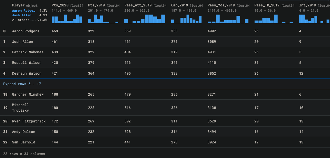
merged_with_madden = pd.merge(merged, combined_madden, how="left").fillna(0)
merged_with_madden
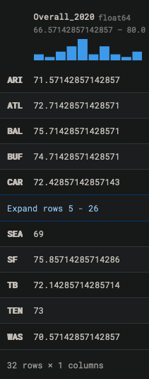
Next, I need to determine the strength of each QB’s offensive line. This was a little bit trickier as I could not find ready-made data from this aggregated per team. Instead, I used the madden data again to aggregate the overall rankings of offensive line positions per team. I focused on the top 8 OL players per team, to take into account depth but also not let 3rd string players throw off the average.
# LT, LG, C, RG, RT
ol_positions = ["LT", "LG", "C", "RG", "RT"]
ol_2020 = pd.read_csv("FF_2021/2020_player_team_full.csv")
ol_2020 = ol_2020[ol_2020.Position_2020.isin(ol_positions)].replace({"Team_2020": team_name_to_short_form})
ol_2020

ol_2020_rankings = pd.merge(ol_2020, madden_2020, on=['Player'], how="left").drop(columns=["2020_Age", "2020_Injury"]).rename(columns={"2020_Overall": "Overall_2020"})

ol_2020_rankings = ol_2020_rankings.groupby(['Team_2020']).head(7).reset_index(drop=True)
ol_2020_overall = ol_2020_rankings.groupby(['Team_2020']).mean()
ol_2020_overall

I used this data and pulled it into another CSV to simplify the code. I merged in the rankings with the main player dataframe to create the final merged dataframe:
ol_2020_overall = pd.read_csv("FF_2021/ol_2020_overall.csv")
merged_with_madden = merged_with_madden.rename(columns={"Team_2020" : "Team"})
merged_with_madden_and_ol = pd.merge(merged_with_madden, ol_2020_overall, on=['Team'], how="left").drop(columns=["Team"])
merged_with_madden_and_ol

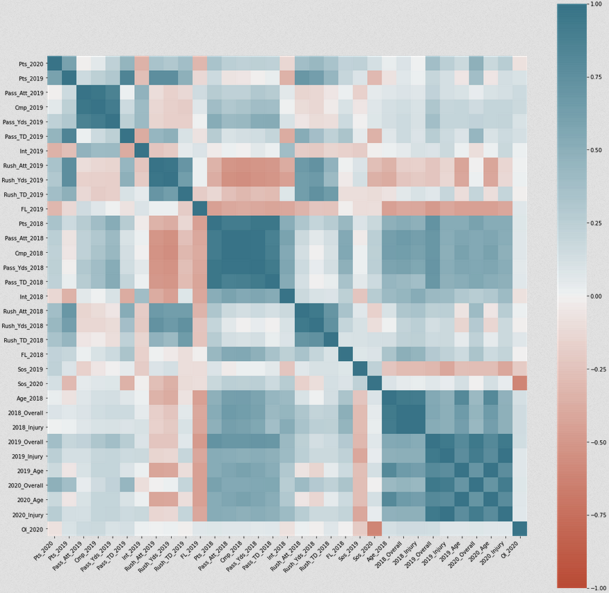
Then, I explored the data using a correlation matrix.
corr = merged_with_madden_and_ol.corr()
plt.figure(figsize=(20,20))
ax = sns.heatmap(
    corr,
    vmin=-1, vmax=1, center=0,
    cmap=sns.diverging_palette(20, 220, n=200),
    square=True
)
ax.set_xticklabels(
    ax.get_xticklabels(),
    rotation=45,
    horizontalalignment='right'
)

Strength of schedule does weakly negatively correlate with points as expected. A positive injury rating (less likely to be injured) correlates positively with points as well. Madden overall rankings are good predictors of fantasy points as well.
With all the data I need, I can once again use a GradientBoostingRegressor to evaluate our new model.
# Get the training data
train_data = merged_with_madden_and_ol.drop(["Player", "Pts_2020"],axis=1)
target_label = merged_with_madden_and_ol["Pts_2020"]

n_features = train_data.shape[1]
x_train, x_test, y_train, y_test = train_test_split(train_data, target_label, test_size = 0.30)

clf = ensemble.GradientBoostingRegressor(n_estimators=50, random_state=0)

space  = [Integer(1, 15, name='max_depth'),
          Real(10**-5, 10**0, "log-uniform", name='learning_rate'),
          Integer(1, n_features, name='max_features'),
          Integer(2, 100, name='min_samples_split'),
          Integer(1, 100, name='min_samples_leaf')]

@use_named_args(space)
def objective(**params):
    clf.set_params(**params)

    return -np.mean(cross_val_score(clf, x_train, y_train, cv=5, n_jobs=-1,
                                    scoring="neg_mean_absolute_error"))

clf_gp = gp_minimize(objective, space, n_calls=50, random_state=0)

print(clf_gp.fun)
print("""Best parameters:
- max_depth=%d
- learning_rate=%.6f
- max_features=%d
- min_samples_split=%d
- min_samples_leaf=%d""" % (clf_gp.x[0], clf_gp.x[1],
                            clf_gp.x[2], clf_gp.x[3],
                            clf_gp.x[4]))

clf2 = ensemble.GradientBoostingRegressor(n_estimators=50, random_state=0, max_depth = 1, learning_rate=1.0, max_features=32, min_samples_split=2, min_samples_leaf=1)
clf2.fit(x_train, y_train)
clf2.score(x_test, y_test)
This produced a value of 0.2-0.7, which is higher than the previous model but still wildly variable and too inaccurate.
Next, let’s look at the relative importance of each feature using permutation importance and see if we can potentially improve the model by dropping redundant features.
perm = PermutationImportance(clf).fit(x_test, y_test)
eli5.show_weights(perm, feature_names = x_test.columns.tolist())
0.8091 ± 0.6043 	2020_Overall
0.3480 ± 0.3964 	Int_2019
0.2457 ± 0.3458 	Pass_TD_2018
0.0936 ± 0.4800 	Int_2018
0.0522 ± 0.4518 	Rush_Yds_2018
0.0394 ± 0.0429 	Cmp_2019
0.0360 ± 0.0461 	FL_2019
0.0251 ± 0.0286 	2020_Age
0.0205 ± 0.0097 	Age_2018
0.0037 ± 0.0096 	Pass_TD_2019
0.0014 ± 0.0040 	2019_Injury
0.0010 ± 0.0047 	Ol_2020
0.0001 ± 0.0011 	Pass_Yds_2018
0.0001 ± 0.0070 	Cmp_2018
0 ± 0.0000 	2019_Overall
0 ± 0.0000 	2019_Age
0 ± 0.0000 	2018_Injury
0 ± 0.0000 	Pts_2018
0 ± 0.0000 	Rush_Att_2019
0 ± 0.0000 	Sos_2019
Not too suprising, but the madden 2020 overall rating for each player is by far the most important feature in predicting fantasy performance. Interestingly enough, the interceptions from the 2019 season was the second most important feature, with several 2018 stats following after. Offensive line strength was not a strong predictor, which implies that either my OL strength calculations are not great, or it’s not a major factor.
To see if just focusing on key features will improve the model, I created a new GBR with just the key features.
merged_key_features_only = merged_with_madden_and_ol[["Player", "Pts_2020", "2020_Overall", "Int_2019", "Pass_TD_2018", "Int_2018", "Rush_Yds_2018", "Cmp_2019", "FL_2019", "2020_Age"]]

train_data = merged_key_features_only.drop(["Player", "Pts_2020"],axis=1)
target_label = merged_key_features_only["Pts_2020"]

n_features = train_data.shape[1]
x_train, x_test, y_train, y_test = train_test_split(train_data, target_label, test_size = 0.30)

clf2 = ensemble.GradientBoostingRegressor(n_estimators=50, random_state=0, max_depth = 15, learning_rate=.1, max_features=2, min_samples_split=50, min_samples_leaf=50)

clf2.fit(x_train, y_train)
clf2.score(x_test, y_test)
This produced values slightly worse that the previous model with more features.
Depending on the hyperparameter tuning and the slicing of training data, this produced an R^2 value of 0.2-0.7, which is higher than the previous model but still wildly variable and too inaccurate.
There is additional in-season aggregated data we can look into, but stepping back again I think I have hit a fundamental wall just looking at overall season aggergated data. There were only 23 QBs that had valid stats going back 2-3 years, and we’re looking at 34 total columns of data in our final merged dataframe. Even if I do some more parameter tuning (for example we can drop 2018 and 2019 ages, or drop most of the 2018-2019 individual stats since they correlate to 2018-2019 points anyways) there are just not enough rows of data and too much randomness to produce an accurate model.
Looking at other methodologies, such as beer-sheets, they evaluate at a per-game level. I’ll be looking into this next.
Before beginning any feature engineering or ML, it’s necessary to clean up the data first. In this article we work through a real-life example
Discovering several profitable trends that consistently produce positive returns yearly
Leveraging historical performance and spread data to predict what team will cover the spread
昨日はカナダの選挙でした。人気ではありませんでした。
Comparing at the over/under line from 2010 with weather, team ratings, weeks, etc
A review of Matt Rudnitsky’s ‘Smart Sports Betting: How to Shift from Diehard Fan to Winning Gambler’
64% percent of stocks underperform the market and only 6.1% will outperform by 500%+. What makes these outperformers unique?
Using standard QB stats from 2016-2019, teammate ratings, and strength of schedule to predict 2020 fantasy points.
Using standard QB stats from 2016-2019 to compare predicted 2020 fantasy points vs actual performance.
雪が降っていて、桜はアイスクリームみたい
来週、ユダヤの祝日のハヌカーです。
毎年、北米で人気のゲームFantasy Footballをプレイしています。
Available on iOS, Android, BlackBerry, and Web, Red Sea Rescue is a passover themed game using tilt controls to avoid obstacles.
EZ4X is a graphical, automated forex paper trader that allows users to choose techincal indicators and risk tolerance to automatically execute trades on a cu...